Department of Physics and Astronomy

IDL Tutorial: Models and Fitting

Scientific research will very often involve trying to understand a set of observations by comparison to a numerical model. For example, in the Parallax laboratory, we're going to model the apparent motion of a star (actually, the motion of the earth) as a sinusoidal function of time. You'll have a set of observations, the position of the star on the sky as a function of time, that you'll want to fit a sine curve to. The amplitude of the sine curve yields a very important measurement: the distance to that star.

Of course, data are noisy, and so there will be no one unique sine curve that will fit your data; there will be a range of sine curves that will equally well describe the data. More precisely, there will be a range of values for the parameters, the amplitude and the phase, that define the shape of the sine curve. How do we find the appropriate range of acceptable parameters? For parallax, what is the best measure of the distance, and what is its uncertainty?

You should read Norton chapters 13-16 for an overview of the general problem, but here's a simple example. Suppose we have a simple set of measurements of the (1-D) speed of a falling object vs. time (measured using the LabPro devices you saw in PHYS 211/212). We know the slope of this speed function gives the acceleration. Here are the data:

Wow, that falling object was booking by the last measurement. I'd like to see the crater after the impact.

Anyway, load these data into the IDL variables t, s, and ds (here ds refers to the uncertainty in the speed). Plot s vs. t using the following command,

ploterror, t, s, ds, psym=4, xtitle='Time (s)', ytitle='Speed (m/s)', xrange=[-1,10]

Now, let's fit a straight line to the data using robust_linefit (from IDLastro):

coeff = robust_linefit(t, s, sfit, ds, dcoeff)

This function fits the model y = m x + b, a straight line with slope m = coeff[1] and intercept b = coeff[0]. The uncertainty of the fitted parameters is dcoeff, so, for example, the best-fit slope is coeff[1] +/- dcoeff[1]. The resulting model is placed in the variable sfit. To view the model atop the data, enter the following command,

oplot, t, sfit

And, with any luck, the resulting model should make sense. To display the coefficients, try,

print, 'Slope = ',coeff[1], ' +/- ', dcoeff[1], 'm/s^2'

Is the slope consistent with what you would expect near the earth's surface? Did the falling object start from rest?

What is going on?

There's not much to it. Our goal is to tweak some model, y, to match up as closely as possible some set of data, d. How close is close? Well, you'd like the model to be close to a given data point relative to the uncertainty of a given data point. If a given data point has a large uncertainty, we cut the model a little slack. If the data point has a very small uncertainty (the measurement is very accurate), then we want the model to match up well.

In the end, we want to evaluate the quantity chi-squared, which is expressed as,

where the sum is taken over all of the individual data points (subscript i). Here's away to interpret chi-squared in words:

chi-squared = the sum of the distances between data and model, squared, but weighted down by the uncertainties

The smaller the sum, or equivalently the smaller the value of chi-squared, the better the model matches the data. Often the numerical method of finding the best model is iterative:

(1) Make a guess at the correct parameters (for example, the slope and intercept of a line, or the amplitude, period, and phase of a sine wave).

(2) Generate the model y.

(3) Calculate chi-squared

(4) Look at small changes of the parameters (for example, change the slope of the model line slightly, recalculate the model y,), and see if that improves chi-squared.

(5) Repeat until small changes of the parameters no longer reduce the value of chi-squared.

(6) From this procedure, determine which parameters gave the smallest value of chi-squared.

(7) Determine how much you can change the parameters before you get a significant change in chi-squared. (Note that, if you have truly found the minimum chi-squared, any change of the model parameters will increase the value of chi-squared). The result is the uncertainty of the parameters.

In the case of linear models (straight-line models), or models that can be made linear, you can find the parameters analytically - there's no need to iterate. I recommend having a look at chapter 15 in Press et al., Numerical Recipes 3rd Edition, or Bevington, Data Reduction and Error Analysis to learn more about linear fitting. At this stage, we're more interested in operational fitting techniques.

I'm necessarily leaving out a lot of important details. In step (7), what is a significant change of chi-squared? Suppose you have M parameters in your model; in the case of a straight line, M = 2 (slope and intercept). As a reasonable approximation, a significant change of chi-squared for a model is roughly = M.

For example, suppose your best fit chi-squared = 5.2 for a straight-line. To determine the uncertainties, change the slope and intercept until the new value of chi-squared = 7.2 (roughly); the difference between the original slope and the new slope gives a measure of the uncertainty. Of course, this can be done more precisely, and fitting codes will usually do a good job of determining the uncertainties of the model parameters, just as we saw in the example above.

Non-Linear Models

It's often the case that you cannot linearize a model; you cannot modify the data to make the fitting analytical, and you have to resort to an iterative solution as described above. We will be using Craig Markwardt's MPFIT fitting tools (http://www.physics.wisc.edu/~craigm/idl/), which you may have to download if they are not already installed. Try compiling the primary procedure mpfit:

.run mpfit

If it compiles, you are in good shape. If not, you should download a copy to your working directory, or to your personal IDL library.

To give you a feel for how to use mpfit, we're going to fit a simple, non-linear model to noisy data, in this case, a gaussian curve. Recall, a gaussian takes the form,

,

where A is the amplitude of the gaussian, x_c is the location of the center of the gaussian, and sigma measures the width of the gaussian. To be clear: the three parameters of the model are amplitude, centroid, and width.

We'll use a variant form of mpfit called mpfitfun. To use mpfitfun, we have to write a function that will take an array of parameters, values x, and return f(x). Here's one way to write the function, and it will give you a nice shell that you can use to make other functions for mpfitfun.

function jacksgaussian, x, p
; x = abscissae
; p = parameters = [amplitude, centroid, width]
argument = (x - p[1]) / p[2]
gaussian = p[0] * exp(-argument^2)
return, gaussian
end

Now, load the data in noisygaussian.txt into variables, x, y, and dy (dy contains uncertainties). Here's a plot for comparison.

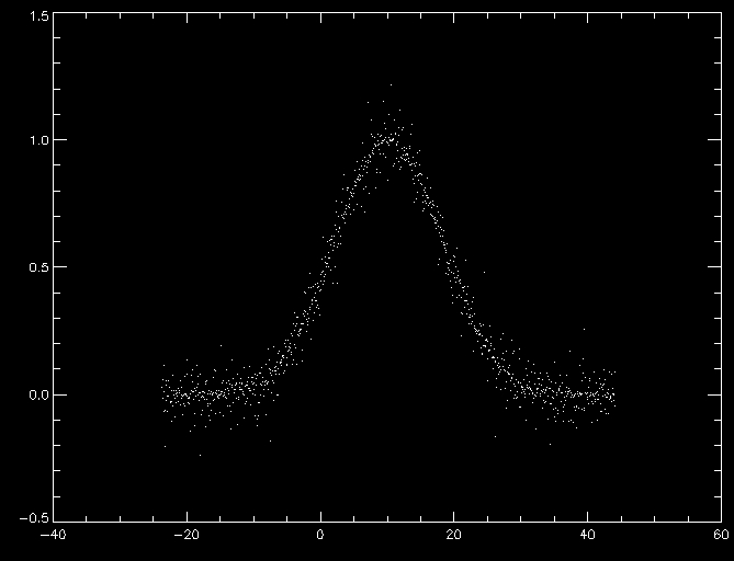
Now, to fit these data, make the file jacksgaussian.pro as defined above. Since mpfitfun is iterative, we need to give it an initial guess as to what the parameters should be. From inspection of the plot, above, it looks like the centroid is at about x = 10, the width is ~ 10 units in x, and the amplitude looks to be about 1. So, our starting parameters can be defined,

startparms = [1.0, 10.0, 10.0]

Then, run mpfitfun, and watch as it iteratively improves our initial guess to minimize chi-squared.

parms = mpfitfun('jacksgaussian', x, y, dy, startparms, perror = dparms, yfit=yfit)

The best fit parameters will be stored in parms, and their uncertainties will be stored in dparms. The model prediction for each value of x is stored in yfit. You can compare the model with the data by overplotting:

plot, x, y, psym=3

oplot, x, yfit

While mpfitfun is running, it will give you some interesting statistics about each iteration, namely, the current parameter values, the current value of chi-squared, and the DOF, or degrees of freedom, where DOF = # of data points - number of model parameters. In general, for a model to be a valid representation of the data, you would expect chi-squared ~ DOF. Is that the case for this particular modelfit?

Use of Double Precision

Sometimes iterative fitting techniques will hang on a bad solution because the numbers are stored in the computer with insufficient precision; standard floating-point precision is 7 significant figures (in decimal numbers). In reality, there may be a better solution, but the computer cannot find it because rounding to 7 significant figures precludes finding a better solution.

To get around that problem, it's worth working in double precision, where you get roughly 16 significant figures (these are rough conversions because, of course, the computer uses binary numbers).

To use mpfitfun in double precision, just send the initial guesses in double precision.

startparms = [1.0d, 10.0d, 10.0d]

Notice that all I did was to add a "d" at the end of each decimal number.

Advanced Fitting: Controlling and Limiting the Parameters

The mpfit routines allow for some additional control over the fitting. For example, what if you had some information that the amplitude of the gaussian had to be greater than zero? What if you knew that the centroid was precisely 10.2? You want to provide the fitting routine with this information so that it doesn't go off on the wrong path.

Control information is passed through the structure variable parinfo, which is easier to learn by example rather than by explanation (there is detailed documentation in the mpfitfun.pro file). Here's an example of parinfo for the situation I just described.

parinfo = replicate({value:0.0, fixed:0, limited:[0,0], limits:[0.0,0.0]}, 3)

This statement initializes the control array to its defaults; i.e., all parameters vary freely. The last number is the number of parameters in your model; for the gaussian, 3.

Now, we want to fix the amplitude to be greater than 0.

parinfo[0].limited[0] = 1; parameter 0, the amplitude, has a lower bound

parinfo[0].limits[0] = 0.0; do not accept values less than zero

Now lets force the centroid to be 10.2.

parinfo[1].fixed = 1

parinfo[1].value = 10.2

By the way, it's a good idea not to use startparms if you are going to use parinfo. Instead, set your initial guesses in parinfo.

parinfo[0].value = 1.0

parinfo[2].value = 10.0

And, of course, we've already set parinfo[1].value when we fixed the centroid.

Now, retry the fit and see what happens.

startparms[1] = 10.2

parms = mpfitfun('jacksgaussian', x, y, dy, perror = dparms, yfit=yfit, parinfo=parinfo)

Exercise

Here's a new data file: 'datatomodel.txt'. Write your own model function to fit the data using mpfitfun.

Back to Index

Next Tutorial

Last modified by Jack Gallimore.