Correlated uncertainties -- Two approaches
Introduction
Consider the oft-encountered problem of calibrating an instrument. To be specific, let's consider the simple case in which you are calibrating a spectrometer, using a set of spectral lines with known wavelengths $\lambda_i$. You measure the pixel number $p_i$ on the CCD array of the spectrometer for each of the lines, and each of these measurements has an associated uncertainty $\sigma_i$ (uncertainties in the known wavelenths is assumed to be negligible). Let's also assume that a preliminary analysis suggests that data is well-modeled by a linear relationship between $\lambda$ and $p$ (it's straightforward to generalize to more complicated relationships).
In an experiment in which this calibration data is to be used, the value of the pixel number measured for a spectral line of unkown wavelength. Let's call the measured value of the pixel number for this unknown line $p^\ast$, and the associated uncertainty $\sigma^\ast$.
The question is: How do we determine the best value, including the uncertainty, for the unknown wavelength $\lambda^\ast$?
Naive (and incorrect approach):
Since there is good evidence for a linear relationship between $p$ and $\lambda$, why not simply fit $\lambda$ as a function of $p$, and use the linear relationship: $\quad \lambda^\star = \mbox{slope}\times p^\star + \mbox{intercept}$?
Whle this approach can give a "quick and dirty" estimate for $\lambda^\ast$, it is fundamentally flawed. All of the standard fitting routines we have used are based on the assumption that the uncertainties are all in the dependent variable. They can't be expected to handle uncertainties in the independent variable corrrectly, and they can't give any information about the uncertainty in the slope, the intercept or $\lambda^\ast$.
Discussion of better approach, and correlated uncertainties
To get good information about the relationship between $\lambda$ and $p$ we must fit the function
$$ p = m\lambda + b $$to find values of $m$ and $b$, and then invert this function to find
$$ \lambda^\ast = \frac{1}{m}(p^\ast - b). $$In determining the uncertainty $\sigma^\ast$ in the measurement of the unknown wavelength there is an additional complication: the values of $m$ and $b$ determined by the fitting function are correlated. To understand correlation, consider the following cartoon.
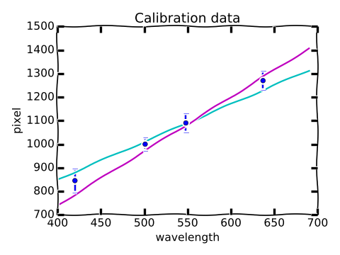
The fact that there is an uncertainty in the slope and the intercept of the best-fit line is captured in the graphic by the fact that there is a range of "reasonable" lines from which determine the "best" by minimizing the $\chi^2$ statistic. In looking at the illustrated extreme cases of "reasonable" lines, we see that the teal line has a low slope, but a relatively high intercept, while the purple line has a high slope, but a relatively low intercept. It is extremely unlikely that the data is fit by a line with a slope as large as that of the purple line, and an intercept as large as the teal line; such a line would lie above all of the data points. It is in this sense that the uncertainties in the slope and intercept are said to be correlated.
One other feature to deduce from the cartoon is that a measurement of a pixel value $p^\ast$ for the unkown spectral line near 1100 will give a relatively small range of "reasonable" values for $\lambda^\star$, while a $p^\ast$ measurement of 1300 will give a much larger uncertainty in $\lambda^\star$.
In this notebook we will explore two approaches to the quantitative determination of the uncertainty in values of the wavelength $\lambda^\star$ using a model data set.
- In the first approach we will use Monte Carlo methods to simulate data sets that are statistically equivalent to the calibration data. We won't use any propagation-of-errors rules, or combination-of-uncertainty rules; we'll just simulate lots of "experiments" and look at the spread in the outcomes.
- In the second approach we show how to generalize things when simple rules for uncorrelated uncertainties break down. For example, when uncertainties are correlated, $$ \alpha_\text{total} \neq \sqrt{\alpha_1^2 + \alpha_2^2 + \alpha_3^2 +\dots}. $$ Simple cases of how to handle correlated uncertainties are discussed in Section 7.3 of Hughes and Hase. In this notebook we will use a computer to calculate autmatically quantities like those given in Table 7.2 using information returned by the LinearModelFit() function.
NOTE: In the notebook below I make the transition from wavelength and pixel to the more general $x$ and $y$:
$$ \lambda \longrightarrow \verb+x+,\quad p \longrightarrow \verb+y+,\quad \delta_p\longrightarrow \verb+u+ $$$$ p^\star \longrightarrow \verb+ystar+, \quad \delta_{p^\star} \longrightarrow \verb+uystar+ $$Imports and Function Definitions
import matplotlib.pyplot as plt
plt.rcParams['figure.figsize'] = (6.0, 4.5)             # Change default size of plots
plt.rcParams['font.size'] = 14                          # Change default fontsize for figures
plt.rcParams['figure.autolayout'] = True                # Adjusts for changes
# Following line makes plots appear in the notebook. Switch commented line for
# external plots
%matplotlib notebook
#%matplotlib
import scipy as sp
from scipy.linalg import inv, lstsq
Functions from linear_fit_example.ipynb
# Basis functions for linear model:  func = a0*X0 + a1*X1 + a2*X2 + ...
# In this notebook, there are only two basis functions: 1 and x
def basis(x):
    '''Basis functions for linear model

    Functional form:  func = a0*X0 + a1*X1 + a2*X2 + ...
    In this notebook there are only two basis functions: 1 and x
    '''
    X1 = x
    X0 = 0.*X1 + 1. # Need array of len(x)
    return sp.array([X0,X1])

def func(x,a):
    return sp.dot(basis(x).T,a)

# Comments in this function based on the notation of Numerical Recipes
def LinearModelFit(x,y,u):
    '''
    x = list of x values [x0, x1, x2, ...]
    y = dependent variable
    u = uncertainties on y
    '''
    X = basis(x).T    # Basis functions evaluated at all x (the X_j(x_i)) of N.R.)
    W = sp.diag(1/u)  # Matrix with uncertainties on diagonal
    Xw = sp.dot(W,X)  # A_ij of Eq. (14.3.4)
    Yw = sp.dot(y,W)  # b_i of Eq. (14.3.5)
    fit = sp.linalg.lstsq(Xw,Yw)  # lstq returns: best values, chi2, ....
    covariance = sp.linalg.inv(sp.dot(Xw.T,Xw))
    uncertainty = sp.sqrt(sp.diag(covariance))
    return(fit[0],uncertainty,fit[1], covariance)
Linear fit to data for $m$ and $b$
Data to be fit:
# Or: data = sp.loadtxt("file.dat")
# Format:  [[x1,y1,u1], [x2,y2,u2], ... ]   where u1 is uncertainty in y1
data = sp.array([[1, 2.947032612427293, 0.5],
 [2, 6.168779380682309, 0.5],
 [3, 7.1618838821688, 0.5],
 [4, 9.590549514954866, 0.5],
 [5, 11.20657,0.5]])
x = data.T[0]  # separate x values into single array
y = data.T[1]  # separate y alues into single array
u = data.T[2]  # separate uncertainties into single array

ystar = 3.9    # measurement of "unknown" (pixel)
uystar = 0.5   # uncertainty in "unknown"
xfine = sp.linspace(0,6,201)  # "quasi-continuous" set of x's for plotting function
plt.figure(1)
plt.title("data",fontsize=14)
plt.xlabel('$x$')
plt.ylabel('$y$')
plt.axhline(0,color='magenta')
plt.xlim(0,6)
plt.errorbar(x,y,yerr=u,fmt='o');

Perform fit
a, unc, chi2, cov = LinearModelFit(x,y,u)

for i in range(len(a)):
    print("parameter",i,"=", a[i],"+/-",sp.sqrt(cov[i,i]))
print("chi2 =",chi2)
print("reduced chi2 = chi2/(5-2) =",chi2/3)
print("covariance matrix =",cov)
xfine = sp.linspace(0,6,201)  # "quasi-continuous" set of x's for plotting of function
plt.figure(2)
plt.title("data with best fit line",fontsize=14)
plt.xlabel('$x$')
plt.ylabel('$y$')
plt.axhline(0,color='magenta')
plt.xlim(0,6)  # Pad x-range on plot
plt.errorbar(x,y,yerr=u,fmt='o');
plt.plot(xfine,func(xfine,a));
#plt.show(block=False)

Residuals:
plt.figure(3)
plt.axhline(0,color='magenta')
plt.title('normalized residuals',fontsize=14)
plt.xlabel('$x$')
plt.ylabel('$y$')
plt.grid(True)
plt.scatter(x,(func(x,a)-y)/u);

Results from linear fitting
slope and intercept:
b,m = a
print("slope = ",m,"+/-",unc[1])
print("intercept =",b,"+/-",unc[0])
Value for "unknown": $\quad x^\ast = \frac{1}{m}(y^\ast - b) $
b, m = a   # For use later
xstar = (ystar - b)/m
print("unknown 'wavelength' =",xstar,"+/- ?")
The fitting function does not give a value for the uncertainty in $x^\ast$.
Uncertainties I: Monte Carlo approach
"Offered the choice between the mastery of a five-foot shelf of analytical statistics books and middling ability at performing statistical Monte Carlo simulations, we would surely choose to have the latter skill."
Numerical Recipes, W. Press, B. Flannery, S. Teukolsky, and W. Vetterling
In this section we will first redo the determination of the uncertainties in $m$ and $b$ using a Monte Carlo technique. We will then exted this technique to determine the uncertainty in the "unknown" $x^\ast$ (corresponding to the wavelength of the unknown spectral line).
We can generate a simulated data set that is statistically equivalent to the original data set (assuming the model is correct)
ySim = sp.random.normal(m*x + b,u)
y,ySim
Do this many times, fit each of the simulated data sets, and collect the values of $b$ and $m$.
nSim = 1000             # Number of simulated data sets
mSim = sp.array([])     # Array for values of slope from simulated sets
bSim = sp.array([])     # Array for values of intercept from simulated sets

for i in range(nSim):
    ySim = sp.random.normal(m*x+b,u)     # Generate simulated data set
    a = LinearModelFit(x,ySim,u)[0]  # Fit simulated data set
    bSim = sp.append(bSim,a[0])      # Record intercept
    mSim = sp.append(mSim,a[1])      # Record slope
Correlation of $b$ and $m$ evident in "tilt" of graph below
plt.figure(4)
plt.title("Monte Carlo results for slope and intercept",fontsize=14)
plt.xlabel("$b$")
plt.ylabel("$m$")
plt.xlim(0,3)
plt.ylim(1.5,2.5)
plt.axhline(sp.mean(mSim))
plt.axhline(sp.mean(mSim) + sp.std(mSim),linestyle='--')
plt.axhline(sp.mean(mSim) - sp.std(mSim),linestyle='--')
plt.axvline(sp.mean(bSim))
plt.axvline(sp.mean(bSim) + sp.std(bSim),linestyle='--')
plt.axvline(sp.mean(bSim) - sp.std(bSim),linestyle='--')
plt.scatter(bSim,mSim,marker='.',s=0.5);

For fun, we can add $\chi^2_R$ contours to Monte Carlo data
# Set grid in intercept-slope space for evaluation of chi-square
delta = 0.02
mcB = sp.arange(0, 3.5+delta, delta)
mcM = sp.arange(1.5, 3.+delta, delta)
B, M = sp.meshgrid(mcB, mcM)

# Evaluate chi-square at every grid point and subtract minimum value
Z = sp.zeros((len(B),len(B[0])))
for i in range(len(B)):
    for j in range(len(B[0])):
        Z[i,j] = (sp.sum((func(x,sp.array([B[i,j],M[i,j]]))-y)**2/u**2)-chi2)/(len(data)-2)
plt.figure(5)
CS = plt.contour(B, M, Z,levels=[1,2,3],colors="k")
plt.title("Monte Carlo results for slope and intercept",fontsize=14)
plt.xlabel("$b$")
plt.ylabel("$m$")
plt.xlim(0,3)
plt.ylim(1.6,2.4)
plt.axhline(sp.mean(mSim))
plt.axhline(sp.mean(mSim)+sp.std(mSim),linestyle='--')
plt.axhline(sp.mean(mSim)-sp.std(mSim),linestyle='--')
plt.axvline(sp.mean(bSim))
plt.axvline(sp.mean(bSim)+sp.std(bSim),linestyle='--')
plt.axvline(sp.mean(bSim)-sp.std(bSim),linestyle='--')
plt.scatter(bSim,mSim,marker='.',s=0.5);
plt.clabel(CS);

Simulated data gives no new info about the value of $m$ and $b$, but the spread in the values of does give info about $\sigma_m$ and $\sigma_b$. Agrees with results from least-squares fit. Nothing new, yet.
print("uncertainty in intercept =",sp.std(bSim), "; uncertainy in slope =",sp.std(mSim))
Extend Monte Carlo idea to get information on uncertainty in $x^\star$
- For every simulated data set, pick random $y^\ast$ consistent with measured value
- Use simulated data set and $y^\star$ to determine value for $x^\star$
- Repeat
nSim = 1000             # Number of simulated data sets
mSim = sp.array([])     # Array for values of slope from simulated sets
bSim = sp.array([])     # Array for values of intercept from simulated sets
xstarSim = sp.array([]) # Array for values of xstar from simulated sets

for i in range(nSim):
    ySim = sp.random.normal(m*x+b,u)     # Generate simulated data set
    a = LinearModelFit(x,ySim,u)[0]  # Fit simulated data set
    ystarRan = sp.random.normal(ystar,uystar) # Pick a random ystar
    xs = (ystarRan -a[0])/a[1]       # Calculate simulated xstar
    bSim = sp.append(bSim,a[0])      # Record intercept
    mSim = sp.append(mSim,a[1])      # Record slope
    xstarSim = sp.append(xstarSim,xs)# Record xstar
Results
Uncertainty in $x^\star$ is standard devation of simulated values. This is "new."
print("xstar =",xstar,"+/-",sp.std(xstarSim))
Can also make histogram of Monte Carlo values of $x^\ast$
nbins = 10
low = sp.mean(xstarSim) - 3*sp.std(xstarSim)
high= sp.mean(xstarSim) + 3*sp.std(xstarSim)
plt.figure(6)
plt.xlabel("value")
plt.ylabel("occurences")
plt.title("Histogram; equal sized bins",fontsize=14)
out = plt.hist(xstarSim,nbins,[low,high])

Uncertainties II: Using the covariance matrix
As mentioned above, the total uncertainty in the unknown $x^\ast$ is not given by adding all of the uncertainties in quadrature:
$$ \alpha_{x^\ast}^2 \neq \alpha_{y^\ast}^2 + \alpha_m^2 + \alpha_b^2. $$Rather, it can be shown that the variance in $x^\ast$ is given by
$$ \sigma_{x^\ast}^2 = \left(\frac{\partial x^\ast}{\partial y^\ast}\sigma_{y^\ast}\right)^2 + \left[\left(\frac{\partial x^\ast}{\partial b}\sigma_b\right)^2+ 2\frac{\partial x^\ast}{\partial m}\frac{\partial x^\ast}{\partial b} \sigma_{bm} + \left(\frac{\partial x^\ast}{\partial m}\sigma_m\right)^2 \right] $$where $\sigma_{bm}$ is the covariance between the correlated parameters $b$ and $m$ that is defined in Eq. (7.29) on p. 94 of Hughes and Hase. The variances and the covariance in the square brackets can be collected in the covariance matrix:
$$ \Sigma \equiv \left(\begin{array}{cc} \sigma_b^2 & \sigma_{bm} \\ \sigma_{bm} & \sigma_m^2 \end{array}\right) , $$which is one of the things returned by the least square fitting procedure used above. Writing the variance in the value of $\lambda^\ast$ in terms of the covariance matrix and the row vector $\nabla \lambda^\star$, in which the derivatives are taken with respect to $b$ and $m$ and evaluated at the best fit values of these parameters, gives
$$ \sigma_{x^\ast}^2 = \left(\frac{\partial x^\ast}{\partial y^\ast}\right)^2\sigma^2_{y^\ast} + (\nabla x^\star)\cdot \Sigma\cdot (\nabla x^\star)^\text{T} $$import numdifftools as nd # Module for numerical evaluation of derivatives
def f(p):       # Function for calculation of lambda-star from b and m
    return (ystar-p[0])/p[1]
def f2(ystar):  # Same function, but ystar is the variable
    return (ystar-b)/m
best = sp.array([b,m])
unc_p = nd.Derivative(f2)(ystar)*uystar
beta = nd.Gradient(f)(best)          # Gradient of lambda-star evaluated at (b,m)
unc_mb = sp.sqrt(beta@cov@beta.T)    # As of python 3.5, @ symbol gives matrix multiplication
unc_xstar = sp.sqrt(unc_p**2 + unc_mb**2)
print("The value of the unknown wavelength is",xstar,"+/-",unc_xstar)
Version details
version_information is from J.R. Johansson (jrjohansson at gmail.com)
See Introduction to scientific computing with Python:
http://nbviewer.jupyter.org/github/jrjohansson/scientific-python-lectures/blob/master/Lecture-0-Scientific-Computing-with-Python.ipynb
for more information and instructions for package installation.
If version_information has been installed system wide (as it has been on Bucknell linux computers with shared file systems), continue with next cell as written. If not, comment out top line in next cell and uncomment the second line.
%load_ext version_information

#%install_ext http://raw.github.com/jrjohansson/version_information/master/version_information.py
%version_information scipy, matplotlib