Ben Vollmayr-Lee
(Those from Baseball Primer: this is a Fanhome post from some time in the spring of 2002. The formatting isn't complete, but hopefully it should be readable.)
I use ``pythagorean'' in quotes because I want to speak more generally about the idea of taking RS (runs scored) and RA (runs allowed) and predicting a team's winning percentage. My view is that concepts are more important than formulas, and the relative success of different formulas can tell you things about the concepts.
First, if all we know about a team is that RS = RA, then our best guess at their winning percentage has to be 0.5 (or 1/2). From that starting point let's ask: how much does winning pct go up as run scoring is increased? Let's introduce
           RS
     x = ------- = fraction of runs a team scores
         RS + RA
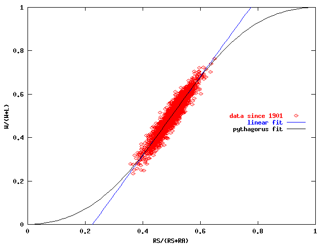
and p = winning percentage. We know p=1/2 for x=1/2. It's useful to look at a plot of p versus x for each team since 1901:
You'll notice the main feature of the data is a linear variation with a slope greater than 1. If we wanted to fit this data as such, we could take a formula like
                       1             1
     Linear fit:  p = --- + n*( x - --- )
                       2             2
Here n is the slope (and turns out to be quite connected to the pythagoras exponent), and a best fit gives n=1.819, so roughly two. This is a useful rule of thumb to know by heart and keep in your head:
Whatever excess (above one-half) of the fraction of runs scored, multiply it by two to get the excess (above one-half) of the winning percentage.
So a team which scores about 55% of the runs will win about 60% of the games. Why a factor of two? That involves the variation in runs per game in baseball, the variation in quality of starting pitching from ace to 5th starter, and the variation of quality of teams in the majors. So there is no easy derivation, though it is interesting to isolate different factors and see what effect they have on this slope. And actually it should be slightly less than two, so you might want to remember the rule of big toe:
Same rule as above, but multiply by 1.8 instead.
What does this have to do with pythagoras? I can write pythagoras as
                         RS^n          x^n
     Pythagoras: p = ----------- = -------------
                     RS^n + RA^n   x^n + (1-x)^n
That second step might not be obvious, but if you divide top and bottom of the original formula by (RS + RA)^n you can derive it. Now what does this have to do with a linear fit? Plenty. We can re-write p as an expansion in powers of (x-1/2) by a process called Taylor expansion (or you can do it with a lot of mucky algebra - you'll get the same answer), and we get
                       1            1      4 n (n^2-1)       1
     Pythagoras:  p = --- + n (x - ---) -  ----------- (x - ---)^3 + ...
                       2            2           3            2
We find only odd powers of x-1/2, which is due to a symmetry in the pythagorean (or any valid) formula, that a team scoring 55% of the runs and a team scoring 45% of the runs should have winning percentages that sum to 1. Notice that the exponent of the pyth formula IS the linear coefficient. The cubic term is negative and represents a type of diminishing returns in winning % versus x. The linear gain eventually curves over, as it must, to give p=1 at x=1 (and by symmetry p=0 at x=0).
How does pythagoras compare to the simple linear formula? First, I do a fit to the data and get n=1.853. I can compare their accuracy to the data since 1901 by measuring the root mean square error in their predicted wins per 162 games. I find
linear fit: 4.226 pythagoras: 4.215
So indeed the diminishing returns made pyth better, but only slightly (so that rule of thumb is a pretty useful thing to remember - the single most important thing to know about this business in my opinion, along with the scale of rms error being about 4 wins).
One problem with pythagoras for determining the diminishing returns is that it uses the same coefficient, n, to fit both the linear and cubic terms (and the quintic for that matter, but it's not very important). We could expect to do better if we allowed the data to pick the cubic coefficient for itself. So let's try a cubic fit:
                     1            1             1
     Cubic fit: p = --- + n (x - ---) + c (x - ---)^3
                     2            2             2
I can give you the parameter values if you're interested, but they're not important. What I find is the fit gives an rms of 4.213, so indeed it does barely better than pythagoras. This is in spite of the fact that the cubic fit, like the linear fit, doesn't give reasonable limits as x goes to 1 or 0. That appears to be less important than getting the leading cubic part of the diminishing returns accurate.
Let's stop and survey the concepts so far:
Okay, up to now we haven't considered at all the average runs per game. As many here know, the degree of offense can affect the pythagorean exponent. So let's explore this some. First, let's check out Pete Palmer's formula (given in Clay Davenport's article). With some algebra you can write this as
                  1      3                1
     Palmer: p = --- +  --- sqrt(r) (x - ---)
                  2      5                2
where x is the same as before and r is the average total runs per game:
       RS + RA
   r = -------
          G
Notice that Palmer's method turns out to be just our linear fit but with a slope that depends on r. If I fit this I get the rms error of 4.220, so it's an improvement over our constant coefficient. But there was no principle behind that number 3/5, so what if I take Palmer's formula and leave the coefficient as a fitting parameter:
                      1                    1
  Palmer + fit:  p = --- + a sqrt(r) (x - ---)
                      2                    2
Now I get 4.204 (with a=0.617403), a significant improvement over all the formulas that didn't include r dependence. And yet there was nothing special about the square root of r. I could use any of the following functions in place of a*sqrt(r):
     a + b r    gives 4.193 (with a=1.262, b=0.06408)

     a + b ln(r)   gives 4.192

     a r^b       gives 4.192
You can see that it doesn't make much difference which we use, so when I want to add run dependence I use the first one above because it's simplest. Notice that all of these formulas, which are linear in x and have no diminishing returns built in, do better than any formula we can make that ignores r. Like pythagoras.
So now another important concept:
Okay, now you can imagine that combining both effects, run dependence and diminishing returns, will do even better still. And indeed it does. A pythagorean formula with the exponent
n = a + b r
gives rms wins of 4.186 (a=1.284, b=0.06541). If I take a formula like Davenport's but re-fit his coefficients I can do slightly better
n = a + b ln(r)
gives rms wins of 4.185. A different cubic fit, which barely made an improvement over pythagoras before, makes essentially no difference here. I think all the work you could possibly do won't improve that by more than a one digit in the last decimal place, so we've basically reached the theoretical upper limit.
When all is said and done, I prefer because of simplicity to use the linear fit/rule of thumb, which can be written as
                     1            1       1     n   RS - RA
    Linear fit: p = --- + n (x - ---) =  --- + (-) ---------
                     2            2       2     2   RA + RA
with n/2 = 0.91. If you want more complexity, it's more important to include the r-dependence than the diminishing returns, so a formula that is still linear in x but with an r-dependent slope is reasonable:
         1                    1      1                b      a
    p = --- + (a + b r) (x - ---) = --- + (RS - RA) (--- + -------)
         2                    2      2                G    RS + RA
with b=0.06408 and a=1.262 (and RS and RA are the season totals, with G games). However, an r-dependent exponent in pythagoras or other diminishing returns fit does slightly better than this last formula, so these will get you that last step towards ``as good as it gets.''
Note: my numbers for wins don't look like those in the Davenport article partly because we use a different data set (he uses some pre-1901 games) but mainly because I calcuate difference in winning pct and then report that as wins per 162 games. Naturally the same error will result in a smaller win variation over 154 games, and he mixes those averages together making his numbers look smaller. It's not important, but I just didn't want anyone confused on this.