Project 3 Discrete Event Driven Simulation

Please refer to the project page for the due dates of the project.

Updated: Please refer back to the discussion of simulation in the lecture, around March 20th. You may also find that the code examples in that discussion can be directly used in the projecct. Here is a link to Prof Meng's notes on the subject and the code examples from the textbook.

1 Academic Integrity

The project falls under the Homework and Projects in the course collaboration policy. Make sure you follow these policies.

2 Objective

The main objective of this assignment is for you to practice and master priority queues and to become familiar with discrete event driven simulations.

3 Introduction

In this extra-ordinary time, many appliance stores and some retail stores are setting up the model of order-online-pick-up-by-the-curb model. The customers can order what they need online, or they can go to the store and shop themselves when the number of customers in the stores are fewer than the regulations allow. If the customers order online, they can then use the drive-through pick-up lines to retrieve their order. It is important for these stores to assign appropriate number of associates to help the pick-up lines, yet the customers don't have to wait in too long a line for their services. For online stores, the situation is similar in the sense that you need to decide how much computing power and storage to be allocated for your web servers so that they can serve the customers well, yet the equipment dedicated to the service don't go wasted. One way to perform this study is to guess wisely the number of cashiers and helpers the store would need based on some past statistics. For example, last year the store used 100 cashiers and 10 curb-side helpers for each shift. Because this year's situation requires an estimated 20 percent increase in the traffic, you could tell your boss that the store would need 120 cashiers and 12 curb-side helpers. Alternatively, you could use some mathematics formula to calculate these numbers with more accuracy and more what-if analysis, e.g., what if the store gets some very popular items that the customers may flock to the store with increase much more than the average numbers. Yet another and probably more versatile method is to use computer simulation to conduct this type of study where you can change parameters easily and study the results in various different settings.

Discrete event driven simulation is a widely used technique to model and study the behavior of many physical systems similar to the ones described above. These systems may include traffic control system, computer networks, bank operations, super-market check-out counters, and many others. In time-step simulation, as we saw in our lab and in our lectures, the simulation is driven by time steps. At each clock tick, e.g., minute or second, the current status of the system is examined and events are handled as they occur at that moment of time. In this type of simulation, the program has to step through every tick of time, whether or not anything is happening at that moment. This is not very efficient computation. In event-driven simulation, the simulation is driven by the sequence of events that are taking place in the system. That is, the simulation system takes actions only when an event is happening. We added the term discrete to the type of simulation we would like to conduct because in the simulations we are developing, the time when events could happen is discrete, not continuous. That is, an event takes place at a discrete time point, e.g., 3, 5, 20, and others, not in a continuous range, e.g., (3, 4].

In discrete event driven simulation, events happen in a random fashion at a random time. Every time an event occurs, the program is designed to have a mechanism to handle this type of event. For example, if we take a snapshot of the operations of a bank branch office, we may see at time 10:13 a.m., a customer arrives (Event A), the customer receives the service from a bank teller at 10:17 a.m. (Event B), the customer completes its transaction at time 10:25 a.m. (Event C), and the customer leaves the branch office at 10:32 a.m. (Event D). The following diagram illustrates the four events that take place in a time sequence.

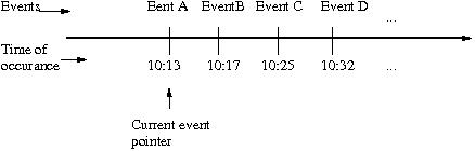
Figure 1: Event driven simulation time line

Instead of checking at every moment, e.g., every minute, if something happens in the system, event-driven simulation schedules for events to take place at certain time in the future and put these events in an event queue. The event queue is ordered by the time when the events are happening. Thus an event queue is a priority queue using the event time as the priority value. When new events take place, they are inserted into the event queue based on the time when the event will happen. The simulation runs by taking each event off event queue and processing the event accordingly. When processing a current event, some new event may take place in the future as the result. For example, when the first customer arrives at the bank office, four events can be inserted into the event queue (Event A, B, C, and D). Assume a new customer arrives at time 10:20, then this arrival event (Event A1) should be inserted into the event queue after Event B, but before Event C.

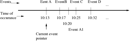
Figure 2: A new customer (A1) arrives at 10:20 a.m.

The general logic of event drive simulation is for the simulation program to process events as they come and schedule future events as appropriate. A general algorithm of a discrete event simulation can be outlined as follows.

generate initial events and insert them into event queue while event queue is not empty and simtime < totaltime: take an event off the event queue set the simtime as the event time process the event (possible generate new events)
Figure 3: General program flow of discrete event drive simulation

3 Simulating Cashiers and Pickup-helpers in an Appliance Store

Your task is to write a discrete event driven simulation to simulate the behavior of cashiers and pickup-helpers in an appliance store when the customers come to the store in certain statistical pattern. The project is divided into two phases. In the first phase, the simulation concentrates on the customers and cashiers (no pickup-helpers). In the second phase of the project, we will add pickup-helpers to the system.

3.1 Phase one: simulating customers and cashiers only

For the first phase, the logic flow is as follows. The customers arrive at the cash register (if online, consider the "register" as the check-out service) at an average rate of 1/λ customers per minute. Each customer spends on average μ1 /2 minutes at the cash register. The inter-arrival time (arrival time between two customers) follows a random distribution between 1 and λ, assuming λ is an integer greater than 1. The time for each customer spent at the cash register is also randomly distributed between 1 and μ1 , assuming μ1 is an integer greater than 1. There are a total number of n register cashiers. For simplicity, we assume that the customers are forming one waiting line when they come to the cash register areas. When a customer comes to the cashier register, if no one is waiting in the waiting line (queue), and if there is a free cashier, the customer receives the service immediately. If someone is already in the waiting queue, the newly arrived customer joins the queue at the end. From the cashier's (the server) point of view, the cashiers keep serving customers until there is no one waiting in the customer queue. That is, every time a cashier finishes serving a customer, they will check the customer queue. If anyone is waiting in the customer queue, the cashier takes the first one off the queue and starts service.

3.2 Phase two: simulating customers, cashiers, and the pickup-helpers

In phase two, we add some complexity to the system. In phase one of the project, a customer leaves the system immediately after the service is completed. (Perhaps these customers take the orders in their own hands?) In phase two, a portion of the customers will go to the pickup-helpers for further service. These pickup-helpers may also help the customers who place their orders online, but pick up their goods at the curb-side. Assume there are a total of m pickup helpers. The time that a customer spends at the curb-side is a random variable with a value between 1 and μ2 . Similar to the service time for cashiers, we assume μ2 is an integer greater than 1. On average, p percent of the customers take the pickup service and 100 - p percent the customers leave the system immediately after paying the cashiers. You may experiment with different values of p, e.g., 0.5 or 0.3.

In both phases of the project, the statistics to be collected is the average waiting time for the customers. For the first phase, the average waiting time at the cashier register is computed. In the second phase of the project, the average waiting time at both the cashier register and the curb-side pickup is computed and reported separately. Your program should also keep the total number of customers arrived, served by the cashiers and the pickup-helpers, as well as the number of customers who are still in the waiting line when the simulation stops.

4 Some Technical Details

This section provides some technical details needed to develop a discrete event driven simulation. Please refer to the Introduction section and Figure 3 for general concepts of discrete event driven simulation.

4.1 Types of events and their handling

One center piece of a discrete event driven simulation is to define the various types of events. In our project, the following events will be needed. You can define these events as a collection of constants in your simulation class.

1. CustomerArrival event: A customer arrives at the cashier registers area at a random time. When a customer arrives, if any cashier is free, the customer starts to receive service immediately. If no cashier is free, the customer joins the single waiting queue. At this moment, your program should generate the next CustomerArrival event. If the current customer arrives at time t, the next customer should arrive at time t + random.randint( 1, lamda ), where lambda is the specified maximum inter-arrival time as an integer. The program should keep a counter of the total customers arrived.


2. CashierServiceBegin event: The customer starts to receive service from a cashier. The cashier is set to be busy. The amount of time the customer spends at the cashier register (scanning all purchased items, computing the total payment, bagging all items, and putting all items into a shopping cart) is also randomly distributed following an exponential distribution random.randint(1 ,mu ), where mu is the specified maximum service time. When a CashierServiceBegin event takes place, an event that the customer service ends should be scheduled at the time the service completes and be put into the event list. When the customer starts to receive service, its waiting time should be computed and be added to the total waiting time.


3. CashierServiceEnd event: When a customer finishes the service at the cashier register, the simulation program should increment the total number of customers who finishes the service with the store. Since now this cashier is free, the program checks to see if anyone is waiting in the customer waiting queue. If someone is waiting, take that customer off the queue and starts the service immediately. If no one is waiting in the queue, the cashier is set to be idle.


4. PickupServiceBegin event: In the first phase of the project, customers who complete the service with the cashiers leave the store immediately. In the second phase of the project, a portion of the customers after finishing with the cashier registers will go to the pickup service to pick up their orders. The pickup service is effectively another service station, similar to the cashier registers. A customer who wants to pick up the order joins the waiting queue if all pickup helpers are busy. If a pickup helper is available, the customer starts the service immediately. The service time is a random variable random.randint( 1, mu1 ), where mu1 is the specified maximum wrapping service time. Similar to that of a cashier register service, when a customer starts the pickup service, the event that the customer ends its service should be scheduled and inserted into the event list. The waiting time in the pickup service should also be computed.


5. PickupServiceEnd event: When a customer finishes their pickup service, the total number of customers who completes this service should also be computed. The simulation checks to see if anyone is waiting in the pickup service queue. If so, the first customer is taken off the queue and starts the service immediately. If no one is waiting, this pickup helper is set to be idle.

4.2 Various queues in the program

The simulation program you are asked to write in this project involves various queues to realize different functionality. Two types of queues are needed, the event queue which is a priority queue whose priority value is the time when an event takes place (event time), and the customer waiting queue at the cashier registers, and the customer waiting queue at the curb-side pickup stations (Phase 2) which is a FIFO queue.

1. Event list (a.k.a. event queue): Events that happen in the simulation are stored in the event list. The events on the even list are ordered by the time when the event should take place in the simulation. (See Figure 2 for an illustration of events happening on the time line.) The main simulation loop (See Figure 3) always takes the first event off the even list and process it as the current event, until either the event queue becomes empty, or the total simulation time is reached. The nodes on the event list should contain three pieces of information, event time, event type, and the customer involved in this event.


2. Waiting queues: All customers who arrive but can't start the service immediately should be put into a waiting queue. In Phase 1 of the project, only one waiting queue exists in the system, the cashier register waiting queue. All customers (cashier registers) share one common waiting queue. In Phase 2 of the project, a waiting queue for the curb-side pickup stations is added. Similar to the cashier waiting queue, all customers who receive the curb-side pickup service share a common queue. These two waiting queues are first-come-first-serve (FCFS) queues. The nodes in these waiting queues should be of the same type as those in the event queue.

4.3 Servers (cashiers and curb-side pickup helpers) and customers

Your program needs two classes of people (see the lecture notes on simulation for defined simpeople), customers and cashiers in Phase 1, and additional class pickup-helpers for Phase 2. Because in our simulation, we will have n cashiers and m curb-side pickup helpers, you need to define an array (or using Python list) of each. It is a good idea to separate these simulation agents (people) from the nodes needed for the event list (see previous section). Define the customers, cashiers, and pickup helpers similar to those in the example from the lectures, but keep the event time separate. The nodes needed for event list and other queues can contain customers as a data member of the object. We can define these nodes as a class called Event.

4.4 Statistics to be collected

The following statistics are to be collected.

1. Average waiting time in the cashier queue (Phase 1 and Phase 2): This value is the total waiting time divided by the total number of customers who receive the service.


2. Total number of customers who completed the service and total number of customers who are left in the cashier waiting queue when the simulation finishes (Phase 1 and Phase 2).


3. In Phase 2, also compute the above two statistics for the pickup station


4. At the end of the simulation, also print such statistics as the total number of cashiers, pickup helpers, total simulation time, and the total number of customers arrived at the store.

3 Test Your Programs and Strategies for Development

Start your program with simple settings and easy to control tests. For example, define the customers, cashiers classes first and test them before using them in the simulation program. When writing the simulation, start the run() method (see the lecture example for which the complete code is given in the course web directory) method with the main while loop, consider what logic should go there in the loop. (See Figure 3.) Concentrate on the simulation logic of customer arrivals and services first before collecting statistics.

It is also a good idea to use print statements throughout the program. For example, when a customer arrives, or when a customer receives and finishes its service, print some information so you can see how the program is running. You can make these printing statements conditional, e.g., define a class variable called debug, set it to be True while debugging, and your printing statements should check if the program is in debugging mode, print the information, if not, don't print anything. When the program is completed, you can set this debug variable to be False so that no extra information is printed. The following is a snapshot of running the program with debugging mode on. (Events between time 2 and 31 are not shown because of limited space.

Simulation starts ... Time 0 : Customer 0 arrived. Time 0 : Customer 0 service starts by cashier 0 Time 1 : Cashier 0 stopped serving customer 0 . ... Time 32 : Cashier 1 stopped serving customer 19 . Time 32 : Customer 20 service starts by cashier 1 ====== Simulation Statistics ======= number of cashier : 2 totalSimTime: 30 interarrivalTime: 2 cashier service time: 5 Number of customers served = 21 Number of customers remaining in line = 1 The average wait time was 1.48 minutes. ===================================== Simulation ends ...
Figure 4: Snapshot of running the simulation

When your program works correctly, you can turn off the debugging mode and print just the summary of the simulation (the last block of the statistics in Figure 4.)

You are asked to test your program with following two sets of parameters for the first phase. You can try other configurations, but submit the results for these two.

1. Number of cashier 2, maximum customer inter-arrival time 2, maximum cashier service time 5, simulation time 1000.


2. Number of cashier 5, maximum customer inter-arrival time 2, maximum cashier service time 14, simulation time 3000.

In the second phase, use the same two sets of parameters as above for cashiers. But add the parameters for the maximum pickup service time of 2 for the both cases. But in the first case, the number of pickup helper is 1, and in the second case, the number of pickup helper is 2.

6 Submission

Submit one zip file for each phase which should include the program and one README.txt file. In the README.txt file, include the result of sample runs and explain your program briefly. Make sure to include the project number and your name in the README.txt files. Submit the zip file for each phase to Moodle separately.

7 Grading Criteria

When grading each of the two phases, we will look for the quality of the program from various aspects as well as the correctness. Here are the grading criteria.

1. Functionality: 60%
1. User-friendly and well-formatted input and output (10%)
2. Correctness of computation (25%)
3. Program satisfies the problem specifications (25%)
2. Organization and style: 30%
1. Program follows object-oriented design approach and contains at least classes for various simulation people, the simulation class itself, and various queues (10%)
2. Variables and functions have descriptive names following Python convention (5%), program contains sufficient amount of docstrings explaining the functionality of its major parts and comments explaining specific actions that blocks of code are performing, each code file has comments on the top including student name, date and file description (5%)
3. Code is structured, clean, organized and efficient. Each python code file that doesn't include the main function contains description of only one class (10%). To earn full grade in this category, avoid leaving commented-out legacy code in your submission.
3. Extraordinary elements, creativity and innovation: 10% This includes anything beyond the provided specification that makes your program stand out.